An Introduction to R

For this section, we will be introducing you to R, a statistical programming language and environment that is widely used in bioinformatics. R is flexible, clear and easy to learn. It also extremely good for producing quick, high quality visualisations of data, which makes it very useful for anyone trying to explore their data. Perhaps the greatest strength of R is its focus on statistics - this makes it an excellent tool for carrying out and learning statistical analysis. R is also used for data analysis beyond evolutionary biology - it forms the basis of data science for companies such as Google, Facebook and Twitter, among many others. If you find yourself wondering why you are learning a programming language, it is worth remembering this point - familiarity with R and scripting will provide you with a very flexible and useful skill.

We believe the best way to get an idea of what R is and what it is capable of is to dive straight in. There really is no better way to learn and understand than to demonstrate the workings of the language to yourself. In this section, we will cover the absolute basics. In the next section, we will learn a bit more about how we can use R to properly manage and manipulate our data. These tutorials will form the basis for how we can apply to R to understanding the genomic data and analyses we have performed.

What to expect

In this section we will:

learn what R is, and start using R as a tool
understand how to handle data structures in R
get familiar with plotting and visualising data
handle datasets and reading in data
loading packages

Getting set up

To begin, you should download and install R from the CRAN. This is the online hub for the R language and it stands for Comprehensive R Archive Network. Be sure to download the correct R installation for your operating system.

We also strongly recommend you install RStudio, a front-end for R. This utility makes working in the R environment a lot more straightforward, standardises things across operating systems and has many helpful features. For the purposes of these tutorials, we will assume you are using RStudio.

With both R and RStudio installed, start Rstudio and we will begin!

Familiarising yourself with the R environment

Now RStudio is loaded, you should see three panels, the console, a panel called environment and one with at least four tabs labelled files, plots, packages and help.

With R, you type commands into the console and then this replies with output. R will operate from within the directory it is started from. This is an important point to remember for later but for now, we will settle with using a single function in order to find out which directory we are in and also get an idea of how this all actually works. In the console, simply type the following:

getwd()

When you type this, you should see the directory that you are in printed in the console. Knowing where R is operating is important for understanding how to read data into the environment, but we will explore this concept more a little later. What is more important to understand is that you typed a function into the R environment, R evaluated it and provided you with an answer. If you want to learn what a function does, you can simply ask R for help. Lets try this with getwd().

?getwd

This should open up a help dialogue. Help pages for functions like this are extremely useful and are very good for getting an idea of what the functions do and how you can use them. There are even examples of how to run them. For a beginner, some of the information in this dialogue will likely seem hard to understand but in time you will be able to read them effectively!

Let’s get used to interacting with the R console. You have already typed a function once and also called for help. You did this at the prompt which should appear like this in the R console.

This is called the prompt because it is waiting for your input in order to respond. Try typing a few numbers like below. What output do you see?

You will probably have noticed that R echoes single numbers back to you, but it also acts like a calculator and actually processes the numbers you enter into it. Characters such as +, -, / and * are operators that mean add, substract, divide and multiply respectively. Using : tells R to print all numbers between the start and end values.

In addition to basic mathetmatical operations such as multiplication, division, addition and subtraction, you can use R to perform logical operations. For example you can ask whether two values are identical or whether one is greater than the other.

# are the values equal?
2 == 2
# is the first value greater than the second?
5 > 10
# is the first value less than or equal to the second
9 <= 10

When you run this code in the console, R will return TRUE or FALSE - denoting whether the logical statements you made are indeed true or false. The examples here are quite trivial, but this is a powerful feature of R (and indeed programming in general) that forms the basis of creating your own functions and performing more complex operations. As a side note, the lines that start with # are comments in our R code - R will not interpret them. These comments are useful when you are writing scripts (see next section) as a reminder for what your code is doing!

R doesn’t just interpret numeric values, it can also handle character information - i.e. words and text. If you type a word in quotes or double quotes, it will repeat it back to you. Like so:

"Hello world!"

Take note of the fact that if you do the same without quotes, it will not work - you will get an error.

Hello world!

As you might already be thinking, typing in single words or numbers like this isn’t of much value, but as you will come to see, this forms the basis of more powerful ways of storing information.

Variables, vectors and assignment

Now that we have interacted with the console and typed some values in, this is a good time to visit the statistical concept of variables.

Numeric vectors

In terms of evolutionary biology and biostatistics, a variable is any characteristic or measurement that varies among individuals. There are many different types of variable - the first type we will examine is numerical. For example, in R, a set of numerical variables would look like so:

c(10, 50, 10, 40)

Let’s breakdown what we did here. The c function is a basic one that you will use a lot - it combines values into what we call a vector. You can think of a vector as one way of storing a set of variables. Take a closer look at c and see that by separating arguments with a comma, you can combine as many values as you want.

Character vectors

Returning to variables, we can also measure categorical variables. These can be things such as names, sex, categories or classes. For example:

c("Mario", "Luigi", "Zelda", "Link")

In R, this is what we would call a character vector. It is identical to the last vector we produced, but with character instead of numerical data.

If we had to continually type in the vectors we want to work on, using R would quickly become extremely ineficient. Luckily we can use the principle of assignment to overcome this. This can be a bit tricky to get your head around at first, but with practice it is straightforward. Let’s take a look at how it works:

# assign variables to objects
a <- c(10, 50, 10, 40)
b = c("Mario", "Luigi", "Zelda", "Link")
# recall them again in the R environment
a
b

We have defined objects - i.e. an object in the R environment we can now refer to with the name we assigned it. What we did here is basically tell R that there are two new objects, one is a, a vector of numeric values and the other is b, a vector of characters. Then to recall the vectors from the environment, all we need to do is type a or b.

Note that there are two ways to assign objects, with <- or with =. Both are correct but for convention, we will use <-

Let’s just check what type of vectors we have here:

class(a)
class(b)

Using the class function, you should see that a and b are numeric and character vectors respectively. When you assign an object, you can call it (almost) whatever you like. However, some basic rules are to avoid the names of functions and to keep names relatively short and clear. When you have to write a lot of code, you will understand why this is valuable!

Factors

As well as numeric and character vectors in R, there is another important type called a factor. A factor is essentially a character vector with different groups or categories (hence it is categorical), which in R are called levels. Let’s take a look at a factor in action:

# create a character vector
myFactor <- c("male", "female", "male", "female", "female", "male")
# turn it into a factor
myFactor <- as.factor(myFactor)
# view the available levels
levels(myFactor)

## [1] "female" "male"

Here we used as.factor to convert our character vector into a factor and levels to look at the different categories. The importance of factors might not be immediately obvious, but as we continue exploring the R language and statistical analysis, you will see they are an extremely useful concept.

Making use of vectors

Now that we have learned about types of vectors and how to assign them, we can start exploring how to manipulate them. This is important for developing an intuition about how R really works.

First of all, we will create two numeric vectors.

x <- 1:10
y <- seq(from = 10, to = 100, by = 10)

What did we do here? Firstly we created x, telling to use all numeric integers (i.e. whole numbers) between 1 and 10. We then used the function seq to create y. seq takes the arguments from and to - i.e. the start/stop values and a third argument, by, telling it how to increment the sequence. See ?seq for more details.

One of the most useful features of working with vectors is the principle of indexing. This lets us extract any value we want from a vector in R. First of all, let’s work out how long these vectors are using the function length.

length(x)

## [1] 10

length(y)

## [1] 10

So we now know there are 10 values in each of these vectors. If we want to view a specific value or range of values, we just need to call the vector object and specify which values in square brackets. For example, to call a single value:

x[5]

## [1] 5

y[5]

## [1] 50

In R, all indices start at 1 (this is important to remember because some languages, such as Python start at 0). If we want to extract values 3-5, we would do the following:

x[3:5]

## [1] 3 4 5

y[3:5]

## [1] 30 40 50

What if you want to extract the third, sixth and ninth values of a vector? Then you can use c, like so:

x[c(3, 6, 9)]
y[c(3, 6, 9)]

What if you want to replace a value in a vector? You can also do this with indices.

# view x
x
# reassign the 5th value
x[5] <- 500
# view x again
x

An important thing to keep in mind when working with vectors is that you can apply an operation to all the variables in a vector at once. Take some time to examine the examples below

x*10
x+10
x-50

Finally it is possble to perform operations on multiple vectors together. Let’s generate two new x and y vectors.

x <- 1:5
y <- 20:24

Now we can perform any numberical operation on them we wish - add, multiply, divide, subtract and so on.

x*y
x+y
x-y
x/y

Note that for stress-free operations with vectors, like those above, they should be of the same length. If this is not the case, then R will return a warning message. For example.

# two vectors of different length
x <- 1:5
y <- c(10, 100)
# multiply them together
x*y

## Warning in x * y: longer object length is not a multiple of shorter object
## length

## [1]  10 200  30 400  50

The operation worked, but it produces a warning - you can also see that R will reuse the second vector. So here the first value of x is multiplied by 10, the second by 100, the third by 10 and so on.

Variables in statistics

So far with R, we have learned about categorical and numerical values. In more traditional statistical terms, there are other ways to classify these two major types. For example, categorical variables are often referred to as qualitative and are either nominal or ordinal. Ordinal categorical variables have an order, such as life stage in a species. In contrast, nominal categorical variables have no order, such as sex or karyotype.

Numerical variables are straighforward but can also be split into different classes. They can be continous, for example height or weight. They can also be discrete as in they are integers or real numbers. Number of individuals is an example of such a discrete numerical variable - it does not make sense for there to be 2.5 individuals!

Basic plotting and visualisation

The versatility of plotting in R is one of the language’s most attractive and important features. Visualising data is essential for properly understanding and exploring data - it can help you identify measurement error, understand how your data will fit a test or purpose and most importantly of all, point towards interesting hypotheses to test.

A very simple scatterplot

The easiest and most straight forward plot to generate in R is a scatterplot - i.e. variation between values on two different vectors. To plot this, we need to create two numeric vectors like so.

x <- 1:10
y <- 21:30

We can then simply use the plot function to plot them quickly and easily.

plot(x, y)

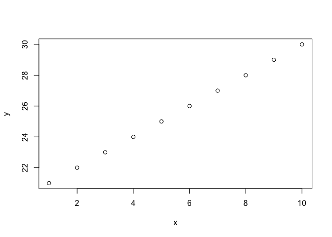
Perhaps not the prettiest plot you’ll generate, but extremely easy to generate! Later, we will learn ways to alter the appearance of a plot.

Visualising a distribution

To demonstrate how R can help you visualise and learn more about statistics, we will focus on the most familiar probability distribution, known for it’s bell-shaped curve, the normal distribution. The first thing we need to do to tackle this concept is generate some data from an ideal normal distribution. For this, we can use the rnorm function.

x <- rnorm(n = 1000, mean = 25.5, sd = 3)

What did we do with rnorm?

n is the number of observations we are sampling; here it is 1000.
mean is the mean (average) value of the distribution; 25.5 here.
sd is the standard deviation of the distribution - this explains the spread of the data around the mean.

This might not make sense immediately, but it will be clearer when we actually visualise the distribution. To do this, we will use the hist function to generate a histogram of the data.

hist(x)

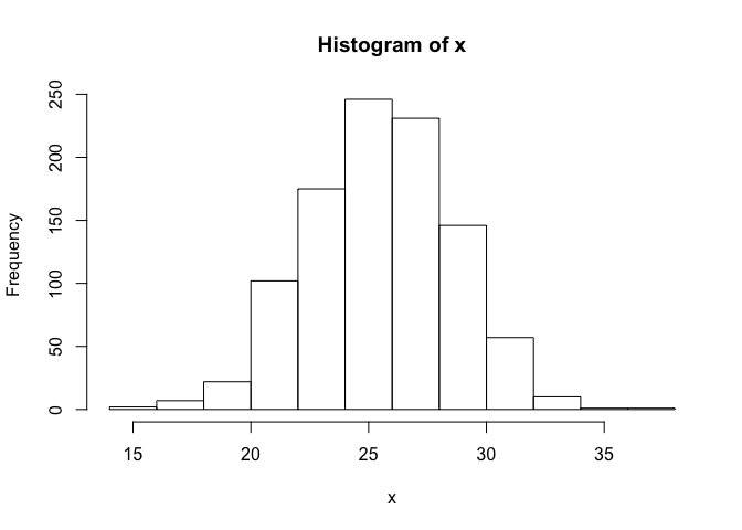
From the histogram plot we generated, you can see the mean is around 25.5, as expected. You can also see that most values from the dataset fall within approximately two standard deviations either side of the mean - i.e. 95% of the distribution occurs here. What this means is that values falling in the tails of the distribution are outliers.

Customising plots

R plots are very easily customised to make them ready for presentations or publications. Let’s generate some data to work with.

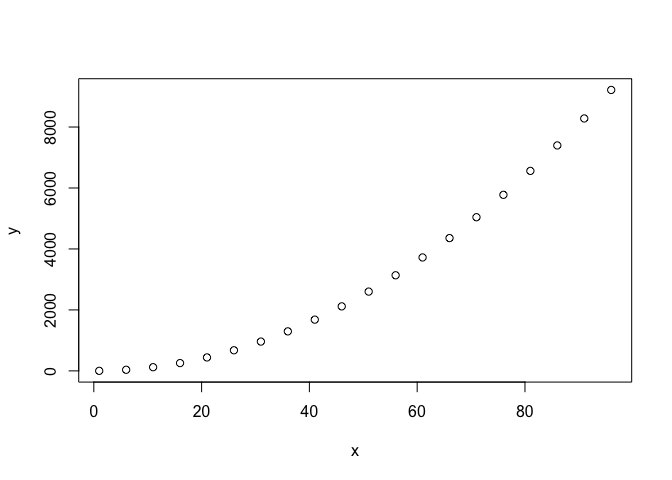
x <- seq(from = 1,  to = 100, by = 5)
y <- x^2

All we did here was square all the values of x to make y. So now we can plot the relationship using an identical plot command to that we used previously.

plot(x, y)

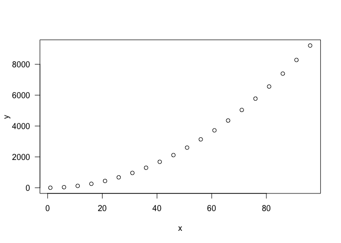
First of all, perhaps we want to change the orientation of the values on the y-axis (maybe you are fussy, like we are). We can do this simply using the las argument.

plot(x, y, las = 1)

Perhaps we want to make the points in our plot a different colour. For example, we can make them red with the col argument like so:

plot(x, y, las = 1, col = "red")

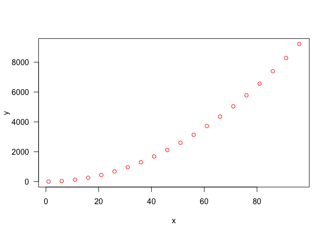
Perhaps we also want to fit a line to our plot? To do that, we use the lines function like this:

plot(x, y, las = 1, col = "red")
lines(x, y)

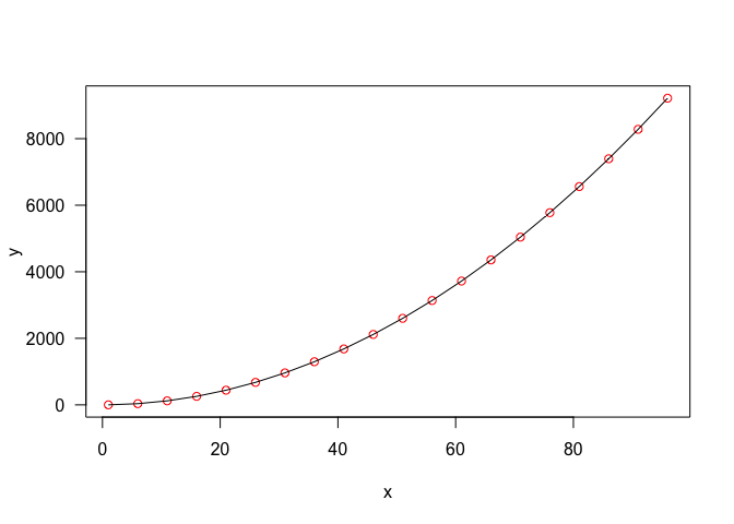
Last of all, we might want to add a title to make sure we know what our plot is actually showing

plot(x, y, las = 1, col = "red", main = "Relationship between x & y")
lines(x, y)

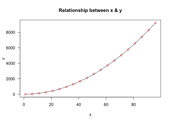
We have only shown a few examples here but it is possible to do so much more with R than these simple plots. To see a few examples, you can use the demo(graphics) call - this will demonstrate plots and the code used to produce them. There are many more indepth R plotting tutorials available online and we provide links to them at the end of this tutorial. There are also plenty of packages such as ggplot2 which allow advanced and more flexible plotting - we will touch on this in the next session.

Moving beyond vectors - matrices and dataframes

We have already learned to store data in R as a vector. We can also access and extract values from vectors. In programming terms, a vector is known as a data structure. In R, there are other data structures beyond vectors which are useful for storing data. In this part of our tutorial, we will turn focus on two similar, but subtly different, structures - the matrix and the dataframe.

Enter the matrix

Matrices essentially store data in rows and columns - similar to a table. You will have undoubtedly come across some manner of a data matrix before, outside of the R environment. The principles are similar within R, you store different variables in different columns and each row represents a different observation.

As with most things, this is a lot easier to get your head around if you start to look at it in practice, so let’s create two vectors and make them into a matrix.

x <- 1:4
y <- 21:24
z <- cbind(x, y)
z

##      x  y
## [1,] 1 21
## [2,] 2 22
## [3,] 3 23
## [4,] 4 24

Here we used cbind to join together x and y as columns. This created a matrix, z. We can use R to verify z is a matrix using the is.matrix function and also learn about the dimensions of our matrix with dim.

is.matrix(z)
dim(z)

When we ask R if z is a matrix, it returns a logical statemnt - TRUE - indiciating it is indeed a matrix. Logical statements are an important concept in programming and we will return to them in the next session.

When we used dim, R responds with two values - the number of rows and the number of columns. A crucial point here is that whenever we refer to matrices, i.e. for extracting data, we first specify the row and then the column. We can also use separate functions such as nrow and ncol to get the same values, like so:

nrow(z)
ncol(z)

Extracting data from a matrix

Now that we know how matrices are built, let’s make a new one and demonstrate extracting some data from it. We will create a matrix in a slighty different way here, using the matrix function.

m <- matrix(1:10, ncol = 2)
m

Here we are telling R to make a matrix with a numeric vector of 1:10, The ncol part of this function tells R that we want two columns. We can also set the rows with nrow but that is calculated implicitly here.

At the moment, our matrix has 1:5 in the first column and 6:10 in the second. We can change the way that the data is entered into the matrix using byrow which is logical argument to the matrix function. If we use the matrix function again, we can see this in action.

m <- matrix(1:10, ncol = 2, byrow = TRUE)
m

Now we can see that the matrix is filled across rows, rather than columns. We are now ready to access data in the matrix. First, we will extract a specific column. Like with vectors, this requires square brackets.

m[, 1]

We can see clearly, that this extracts the first column. Try extracting the second column to demonstrate the principle.

Now what if we want to access a specific row?

m[5, ]

Again, this demonstrates that we first specify the row and then the column. We can actually specify both at once to extract a particular value. For example:

m[4, 2]

This will return 8.

It is worth noting here that all our examples so far have been with numeric matrices. However, it is also possible to make a character matrix. For example

n <- matrix(c("Mario", "Peach", "Link", "Zelda", "Luigi", "Toad"), ncol = 2)

You can treat this matrix exactly as you would if it was numeric. For example:

n[3, 1]

Dataframes

In addition to the matrix, R has a very flexible data structure called a dataframe. Superficially, dataframes and matrices are very similar and indeed, you can use many of the techniques for extracting data from matrices on a dataframe.

However, a matrix can only be completely numeric or completely character based, whereas dataframes allow multiple types of data to be stored in them. To demonstrate this, we will create a basic dataframe from three vectors - one character and two numeric (continous and integer). Let’s generate the vectors first.

name <- c("Mario", "Luigi", "Link", "Zelda")
height <- c(155, 160, 180.3, 180.3)
age <- c(26, 24, 17, 19)

With these three vectors, we can easily create a dataframe using data.frame.

df <- data.frame(name, height, age)
df

You will see immediately that the way a dataframe is displayed is different to a matrix. However, you can extract data from it in a similar way. For example:

df[, 1]
df[3, ]
df[4, 3]

However you can also access the columns of a dataframe directly using their names. To do this, we need to use $. This basically tells R that we are calling the object (here the column) within the dataframe. Try these examples and see:

df$name # nb. this is a factor so will appear differently to the other variables
df$height
df$age

We can actually easy convert our data.frame to a matrix using as.matrix. If we try this, you will see that all the data is converted to character data. You might wonder why we would convert to a matrix but it is occassionally necessary for data operations in R.

as.matrix(df)

With large dataframes, it can be a bit tough to keep track of all the different data types stored. A quick way to get an idea of what one contains is to use str to examine the structure.

# on a data frame
str(df)
# on a matrix - note the shift to all characters
str(as.matrix(df))

R data structures - a summary

With this section, we have become familiar with the fundamental data structures R has to offer. Below is a table summarising the differences among the main three.

Object	Modes	Several modes possible in the same object?
vector	Numeric, character, complex or logical or character	No
matrix	Numeric, character, complex or logical	No
dataframe	Numeric, character, complex or logical	Yes

It is worth noting that there are many other data structures in R and one in particular we have avoided in this introduction is the list. Lists are useful but a little complex for your first ventures with the language - we will cover them in the next session.

Handling datasets in R

Creating vectors, matrices and dataframes is a useful skill, but R’s true power lies in applying your knowledge of these data structures to actual datasets. Obviously we need a way to read data into R in order to access it properly. However, before we learn to do this, we will take sometime to explore some of the many datasets that exist within R.

Example datasets in R

Getting used to handling these datasets is important - they are an excellent way to test out functions, plotting and statistical tests. Use the data function to look at a list of the available datasets.

data()

You can choose any dataset from this list and use the R help to learn more about it. For example, try ?cars or ?iris.

Calling one of these datasets is extremely easy, they are built into R so you can just call them using their names. For example:

head(iris)
str(iris)

Here the head function just shows the first 10 lines of the dataset - giving you an idea of what you are looking at. The iris dataset is a set of measurements from 3 different species of iris and is a classic dataset in biology, measured by Edgar Anderson and used by R.A Fisher to demonstrate fundamental multivariate statistics.

Let’s take a moment here to visualise some of the iris data. Perhaps we are interested in seeing whether petal.width varies between the three species? We can compare the spread of the data between the species using a boxplot. Let’s try the following code:

boxplot(iris$Petal.Width ~ iris$Species, las = 1,
        ylab = "Petal width", xlab = "Species")

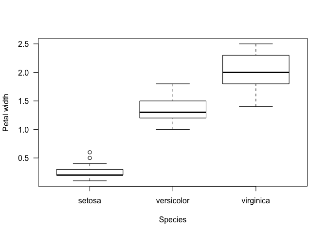
Even if you aren’t familiar with the concept of a boxplot (or more formally, the box-whisker plot), it should be fairly clear from this plot that the three species are quite different in petal width! Let’s breakdown our use of the boxplot function before going into a bit more detail about the plot itself.

What did we do with rnorm?

iris$Petal.Width ~ iris$Species - this argument is a formula in R. It basically means, petal width as a function of species. In plainer terms, we are asking R to show us how petal width varies among species.
las = 1 is just telling the boxplot command to orientate the y-axis horizontally.
ylab specifies the text for the y-axis.
xlab specifies the text for the x-axis.

So what are the boxplots showing us? Essentially, they are displaying the distribution of petal width among the different species of iris. In each case, the black bar indicates the median petal width for the species - i.e. the value lying in the middle of the distribution. The box itself shows the spread of the 25th and 75th percentiles of the distribution - i.e. 50% of the data occurs within the space of the box. The ‘whiskers’ or tails of the boxplot are bit more complicated but essentially represent the extremes of the distribution. Any points occurring beyond these (such as in setosa) are outliers.

Reading datasets into R

As you use continue to use R for day-to-day research and analysis purposes, there will come a time when you want to read your own data in to the R environment. Example datasets are great for teaching and demonstrating examples with code, but obviously they are only examples. Reading in your own data is an essential skill and one that is quite easy to learn.

There are many different ways to read data into R. One of the most obvious is to build the data yourself and we have actually already done this. Consider for example the data.frame we made earlier - this is a way we can create a data structure in R for our own purposes.

df <- data.frame(name = c("Mario", "Luigi", "Link", "Zelda"),
                 height = c(155, 160, 180.3, 180.3),
                 age = c(26, 24, 17, 19))
df

##    name height age
## 1 Mario  155.0  26
## 2 Luigi  160.0  24
## 3  Link  180.3  17
## 4 Zelda  180.3  19

This works if we have only a few observations or a few variables - but could you imagine creating this for hundreds or thousands of observations? It would be a huge waste of your time. Luckily, we can easily read in data using one of the many functions R has at hand.

To demonstrate this, we will read in a simple test dataset that you can get here. Download the data and place it somewhere easily accessible. To make the next few steps straightforward, use the function getwd to identify where on your computer the R environment is running and place the file in the same directory. Once you have done that, use the following code to read in the data.

df2 <- read.csv("./sonic_data.csv", header = T)
df2

##       name height age
## 1    Sonic    100  15
## 2    Tails     80   8
## 3 Knuckles    110  16
## 4   Eggman    185  NA

Here we used read.csv to read in a comma-delimited file. All we needed to tell the function is where to find the file (the first argument, known as the path) and optionally, that the first row of the file contains the names of each of the columns - i.e. header = T.

There are many related functions for reading data in; have a look at the helpfiles for read.table and read.delim for examples. You can also use the RStudio GUI to read in data. On the Environment tab, you can choose the Import Dataset dialogue and read in your data with this interface. This is actually a good way to get used to reading data into R since it will also print the R code used to the console - meaning you can adapt it yourself at a later stage. Have a play around with reading in the sonic_data.csv in this way.

Writing datasets out of R

As well as needing to read data into the R environment, there will also be times when it is convenient to write data out. R is extremely flexible for this kind of operation but to keep things simple here, we will write a data.frame out as a csv file. Using the data.frame we created previously, we use the following code:

df <- data.frame(name = c("Mario", "Luigi", "Link", "Zelda"),
                 height = c(155, 160, 180.3, 180.3),
                 age = c(26, 24, 17, 19))
write.csv(df, "./nintendo.csv")

In its simplest form, write.csv requires just two arguments, the object we want to write out (the data.frame df here) and a path to where we want to write it. As with the read family of functions, there are several related functions to help you write out specific files such as write.table or write.delim.

In, out, shake it all about

Reading and writing data to and from R is quite a convoluted topic as there are many ways to achieve the same thing. Often there are specific packages for handling large datasets or quickly accessing data in special formats. For now, it is sufficient to familiarise yourself with the basics here. In the next session, we will also focus on how to export figures, neatly and cleanly for use in presentations and publications.

Extending your R toolkit - loading packages

When you load R and use the R environment, you are relying on functions to perform analyses and operations. For example, we might want to calculate the mean (i.e. average value) of a vector - to do this we ould use the mean function like so:

height <-  c(155, 160, 180.3, 180.3)
mean(height)

## [1] 168.9

mean is a base function - i.e. it is a basic function that is part of the the R installation. You can see this by typing ?mean and looking at the top of the help page, where you will see mean {base}.

Similarly, we also used the function data earlier to look at the datasets available in the R environment. This is a utils function (check by looking at the help) and is part of the core distribution.

But what if we want to go further than what is bundled with our original R download? Perhaps we want to run a complicated analysis that requires a specific function? Perhaps we just want access to a specific dataset? In that case, we can extend our available R functions by loading packages.

Luckily getting packages in R is extremely straightforward. There are two basic steps - first we need to install a package and then we need to load it into the R environment. We will begin with learning how to install the package ggplot2 - which we will use extensively in the next session.

To clarify the purpose of packages a little more, imagine your available set of R functiosn as being stored in a library (you will soon see the reason for this analogy). If you wish to increase your ‘vocabulary’ of functions, you need to increase the size of your library. By loading a package, you are adding to your library shelf and making it possible for you to do new operations and use new functions.

Installing a package

To install a package, we need to download it from a repository. There are several available for simplicity in these early days of our R adventures, we will use the CRAN - the Comprehensive R Archive Network. The CRAN is the official R repository and the default - so when you install packages, you do not even need to specify it.

Actually, using the function install.packages we can download and install ggplot2 in one quick step. Like so:

install.packages("ggplot2")

For the most of the course, we will be using packages from CRAN. However, when working with genomic data and bioinformatics, we might occasionally also need to use Bioconductor.

The final point to remember here is that we do not need to install the package more than once - it is now present in our R library.

Loading a package

Now that we have downloaded and installed ggplot2, we need to load it in order to actually use it. We can do this easily with the library function.

library("ggplot2")

With ggplot2 loaded, we can look at the ggplot function with ?ggplot. We can also have a look at the package specific data like so:

data(package = "ggplot2")

Now we know how to install and load ggplot2, we are ready to learn to actually use that… but that is for the next session!

Going further

Since R is so widely used, there are many excellent resources out there to help you learn your way. This introduction is just one of them and so here we point you towards some good examples for developing and honing your understanding of working with R.