Filtering and handling VCFs
In the last session, we learned how to call variants and handle VCFs. In this session, we are going to focus on how to filter VCFs. This might seem like a relatively straightforward task but it is actually exceptionally important and something you should spend a lot of time thinking carefully about.
Getting access to the real data
At this point our ‘toy’ dataset breaks down as we do not have enough reads or coverage to call a decent variant set. Recall from the last steps of the last tutorial that most of genotpyes were missing.
To rememdy this, we are going to use a vcf we prepared on your behalf using the full set of reads. To get the full dataset into your directory, use the following commands:
# move to your vcf directory
cd ~/vcf
# copy the data file from the data directory
cp /home/data/vcf/cichlid_full.vcf.gz* ./
This will copy both the vcf and its index to your directory. Let’s take a moment to see how big the file is:
ls -lh *.vcf.gz
You will see that this VCF is 1.5G in size, which is quite large but real analyses with many individuals can run to much larger sizes than this (for instance, we regularly work with VCF files containing hundreds of individuals which are >300 G).
How many unfiltered variants?
One thing we didn’t check yet is how many variants we actually have. Each line in the main output of a vcf represents a single call so we can use the following code to work it out:
bcftools view -H cichlid_full.vcf.gz | wc -l
This command will essentially print every line of the VCF, so if your file is large, it will take quite a long time to run this. For this reason, it might be best to run it inside a screen and then we can check it again later.
Either way, we have close to 8 million variants in our full VCF. That’s a substantial number! But chances are many of them are not useful for our analysis because they occur in too few individuals, their minor allele frequency is too low or they are covered by insufficient depth.
At present, we have applied no filters at all. This is intentional - we want to see what happens when filters are applied. However, it is also a good idea to perform an initial analysis, to get an idea of how to set filters. However as we have just seen, it takes time to perform operations on a large VCF.
For this reason, it is a good idea to subsample our variant calls and get an idea of the general distribution of a few key attributes of the data.
Randomly subsampling a VCF
How can we get an idea of how to set filters? We could just take the first 100 000 variants in our vcf and get an idea of how they look for some basic statistics (i.e. minor allele frequency, depth of coverage and so on). But would this be accurate? What if there is some bias on the first chromosome in the genome and everything there mapped well?
A far better idea is to randomly sample your VCF. Luckily there is a tool to do exactly this and it is part of the extremely useful vcflib pipeline. Using it is also very simple. Here we will use it to extract ~100 000 variants at random from our unfiltered VCF.
bcftools view cichlid_full.vcf.gz | vcfrandomsample -r 0.012 > cichlid_subset.vcf
Note that vcfrandomsample cannot handle an uncompressed VCF, so we first open the file using bcftools and then pipe it to the vcfrandomsample utility. We set only a single parameter, -r which is a bit confusingly named for the rate of sampling. This essentially means the fraction of variants we want to retain.
This will give us at least 95-100 K variants, depending on the random seed used to start the process. This means that everyone in the class should get different random subsets - providing us a nice demonstration for the next step. Before proceeding though, we should compress and index our new subset VCF to make it easier to access:
# compress vcf
bgzip cichlid_subset.vcf
# index vcf
bcftools index cichlid_subset.vcf.gz
Generating statistics from a VCF
In order to generate statistics from our VCF and also actually later apply filters, we are going to use vcftools, a very useful and fast program for handling vcf files.
Determining how to set filters on a dataset is a bit of a nightmare - it is something newcomers (and actually experienced people too) really struggle with. There also isn’t always a clear answer - if you can justify your actions then there are often multiple solutions to how you set your filters. What is important is that you get to know your data and from that determine some sensible thresholds.
Luckily, vcftools makes it possible to easily calculate these statistics. In this section, we will analyse our VCF in order to get a sensible idea of how to set such filtering thresholds. The main areas we will consider are:
- Depth: You should always include a minimum depth filter and ideally also a maximum depth one too. Minimum depth cutoffs will remove false positive calls and will ensure higher quality calls too. A maximum cut off is important because regions with very, very high read depths are likely repetitive ones mapping to multiple parts of the genome.
- Quality Genotype quality is also an important filter - essentially you should not trust any genotype with a Phred score below 20 which suggests a less than 99% accuracy.
- Minor allele frequency MAF can cause big problems with SNP calls - and also inflate statistical estimates downstream. Ideally you want an idea of the distribution of your allelic frequencies but 0.05 to 0.10 is a reasonable cut-off. You should keep in mind however that some analyses, particularly demographic inference can be biased by MAF thresholds.
- Missing data How much missing data are you willing to tolerate? It will depend on the study but typically any site with >25% missing data should be dropped.
Setting up
Before we calculate our stats, let’s make a little effort to make our commands simpler and also to ensure the output is written to the right place. First we need to make a directory for our results.
mkdir ~/vcftools
Next we will declare to variables to save us some typing below.
SUBSET_VCF=~/vcf/cichlid_subset.vcf.gz
OUT=~/vcftools/cichlid_subset
Calculate allele frequency
First we will calculate the allele frequency for each variant. The --freq2 just outputs the frequencies without information about the alleles, --freq would return their identity. We need to add max-alleles 2 to exclude sites that have more than two alleles.
vcftools --gzvcf $SUBSET_VCF --freq2 --out $OUT --max-alleles 2
Calculate mean depth per individual
Next we calculate the mean depth of coverage per individual.
vcftools --gzvcf $SUBSET_VCF --depth --out $OUT
Calculate mean depth per site
Similarly, we also estimate the mean depth of coverage for each site.
vcftools --gzvcf $SUBSET_VCF --site-mean-depth --out $OUT
Calculate site quality
We additionaly extract the site quality score for each site.
vcftools --gzvcf $SUBSET_VCF --site-quality --out $OUT
Calculate proportion of missing data per individual
Another individual level statistic - we calculate the proportion of missing data per sample.
vcftools --gzvcf $SUBSET_VCF --missing-indv --out $OUT
Calculate proportion of missing data per site
And more missing data, just this time per site rather than per individual.
vcftools --gzvcf $SUBSET_VCF --missing-site --out $OUT
Calculate heterozygosity and inbreeding coefficient per individual
Computing heterozygosity and the inbreeding coefficient (F) for each individual can quickly highlight outlier individuals that are e.g. inbred (strongly negative F), suffer from high sequencing error problems or contamination with DNA from another individual leading to inflated heterozygosity (high F), or PCR duplicates or low read depth leading to allelic dropout and thus underestimated heterozygosity (stongly negative F). However, note that here we assume Hardy-Weinberg equilibrium. If the individuals are not sampled from the same population, the expected heterozygosity will be overestimated due to the Wahlund-effect. It may still be worth to compute heterozygosities even if the samples are from more than one population to check if any of the individuals stands out which could indicate problems.
vcftools --gzvcf $SUBSET_VCF --het --out $OUT
With the statistics calculated, take a moment to have a quick look at the output in the ~/vcftools/ directory. We will now need to download our output data onto our local machines in order to work with R.
Examining statistics in R
Setting up the R environment
First load the tidyverse package and ensure you have moved the vcftools output into the working directory you are operating in. You may want to set up an RStudio Project to manage this analysis. See here for a guide on how to do this.
# load tidyverse package
library(tidyverse)
Variant based statistics
The first thing we will do is look at the statistics we generated for each of the variants in our subset VCF - quality, depth, missingness and allele frequency.
Variant quality
The first metric we will look at is the (Phred encoded) site quality. This is a measure of how much confidence we have in our variant calls. First of all, we read in the site quality report we generated using vcftools. We will use the read_delim command from the readr package (part of the the tidyverse) because it is more efficient for reading in large datafiles. It also allows us to set our own column names.
var_qual <- read_delim("./cichlid_subset.lqual", delim = "\t",
           col_names = c("chr", "pos", "qual"), skip = 1)
Take a look at the data when it is read in. You will see that for each site in our subsampled VCF, we have extracted the site quality score. Now we will plot the distribution of this quality using ggplot. Usually, the geom_density function works best, but you can use geom_histogram too.
a <- ggplot(var_qual, aes(qual)) + geom_density(fill = "dodgerblue1", colour = "black", alpha = 0.3)
a + theme_light()
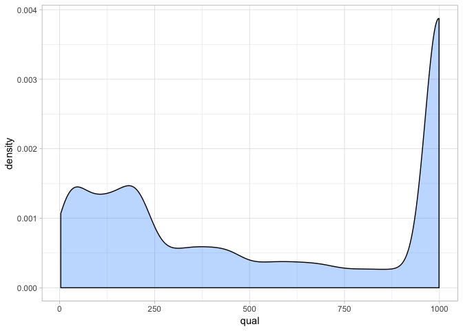
From this we can see that quality scores are actually very high for our sites. Remember that a Phred score of 30 represents a 1 in 1000 chance that our SNP call is erroneous. Clearly most sites exceed this - suggesting we have a lot of high confidence calls. This is most probably because we have sufficient read depth (as you will see in the next section). However since most sites have a high quality we can see that filtering on this is not really going to be that useful.
We recommend setting a minimum threshold of 30 and filtering more strongly on other aspects of the data.
Variant mean depth
Next we will examine the mean depth for each of our variants. This is essentially the number of reads that have mapped to this position. The output we generated with vcftools is the mean of the read depth across all individuals - it is for both alleles at a position and is not partitioned between the reference and the alternative. First we read in the data.
var_depth <- read_delim("./cichlid_subset.ldepth.mean", delim = "\t",
           col_names = c("chr", "pos", "mean_depth", "var_depth"), skip = 1)
Again take a moment to look at the data - mean_depth is our column of interest but note that you can also get a an idea of the variance in depth among individuals from the var_depth column. Once again, we will use ggplot to look at the distribution of read depths.
a <- ggplot(var_depth, aes(mean_depth)) + geom_density(fill = "dodgerblue1", colour = "black", alpha = 0.3)
a + theme_light()
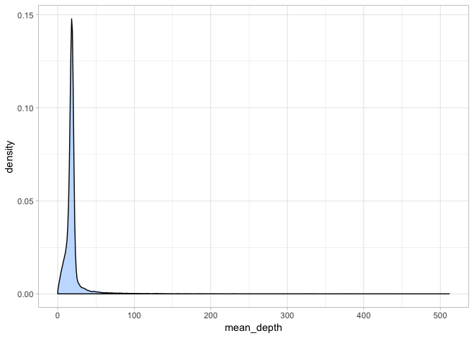
Hmm - this plot is a bit misleading because clearly, there are very few variants with extremely high coverage indeed. Let’s take a closer at the mean depth:
summary(var_depth$mean_depth)
##     Min.  1st Qu.   Median     Mean  3rd Qu.     Max.
##   0.0625  15.1250  17.8750  20.0078  20.0000 511.7500
Since we all took different subsets, these values will likely differ slightly but clearly in this case most variants have a depth of 17-20x whereas there are some extreme outliers. We will redraw our plot to exclude these and get a better idea of the distribution of mean depth.
a + theme_light() + xlim(0, 100)
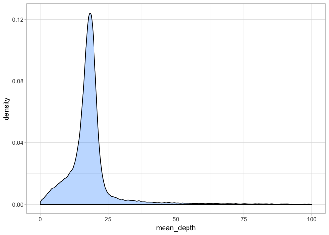
This gives a better idea of the distribution. We could set our minimum coverage at the 5 and 95% quantiles but we should keep in mind that the more reads that cover a site, the higher confidence our basecall is. 10x is a good rule of thumb as a minimum cutoff for read depth, although if we wanted to be conservative, we could go with 15x.
What is more important here is that we set a good maximum depth cufoff. As the outliers show, some regions clearly have extremely high coverage and this likely reflects mapping/assembly errors and also paralogous or repetitive regions. We want to exclude these as they will bias our analyses. Usually a good rule of thumb is something the mean depth x 2 - so in this case we could set our maximum depth at 40x.
So we will set our minimum depth to 10x and our maximum depth to 40x.
Variant missingness
Next up we will look at the proportion of missingness at each variant. This is a measure of how many individuals lack a genotype at a call site. Again, we read in the data with read_delim.
var_miss <- read_delim("./cichlid_subset.lmiss", delim = "\t",
                       col_names = c("chr", "pos", "nchr", "nfiltered", "nmiss", "fmiss"), skip = 1)
Then we plot the data with ggplot2. One thing to keep in mind here is that different datasets will likely have different missingness profiles. RAD-sequencing data for example is likely to have a slightly higher mean missingnes than whole genome resequencing data because it is a random sample of RAD sites from each individual genome - meaning it is very unlikely all individuals will share exactly the same loci (although you would hope the majority share a subset).
a <- ggplot(var_miss, aes(fmiss)) + geom_density(fill = "dodgerblue1", colour = "black", alpha = 0.3)
a + theme_light()
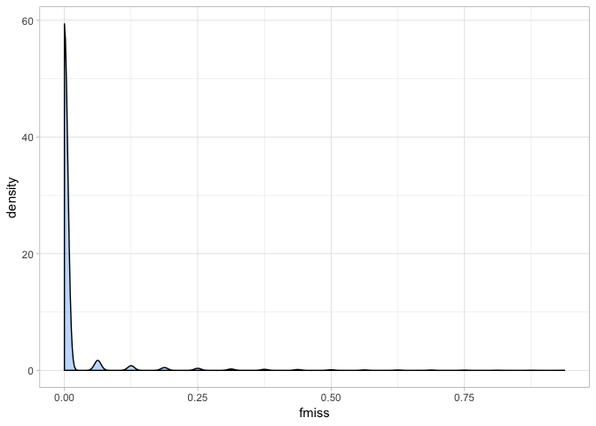
Our cichlid data has a very promising missingness profile - clearly most individuals have a call at almost every site. Indeed if we look at the summary of the data we can see this even more clearly.
summary(var_miss$fmiss)
##    Min. 1st Qu.  Median    Mean 3rd Qu.    Max.
## 0.00000 0.00000 0.00000 0.01312 0.00000 0.93750
Most sites have almost no missing data. Although clearly, there are some (as the max value shows). This means we can be quite conservative when we set our missing data threshold. We will remove all sites where over 10% of individuals are missing a genotype. One thing to note here is that vcftools inverts the direction of missingness, so our 10% threshold means we will tolerate the minimum 90% call-rate (yes this is confusing and counterintuitive… but that’s the way it is!). Typically 75-95% is used.
Minor allele frequency
Last of all for our per variant analyses, we will take a look at the distribution of allele frequencies. This will help inform our minor-allele frequency (MAF) thresholds. As previously, we read in the data:
var_freq <- read_delim("./cichlid_subset.frq", delim = "\t",
                       col_names = c("chr", "pos", "nalleles", "nchr", "a1", "a2"), skip = 1)
However, this is simply the allele frequencies. To find the minor allele frequency at each site, we need to use a bit of dplyr based code.
# find minor allele frequency
var_freq$maf <- var_freq %>% select(a1, a2) %>% apply(1, function(z) min(z))
Here we used apply on our allele frequencies to return the lowest allele frequency at each variant. We then added these to our dataframe as the variable maf. Next we will plot the distribution.
a <- ggplot(var_freq, aes(maf)) + geom_density(fill = "dodgerblue1", colour = "black", alpha = 0.3)
a + theme_light()
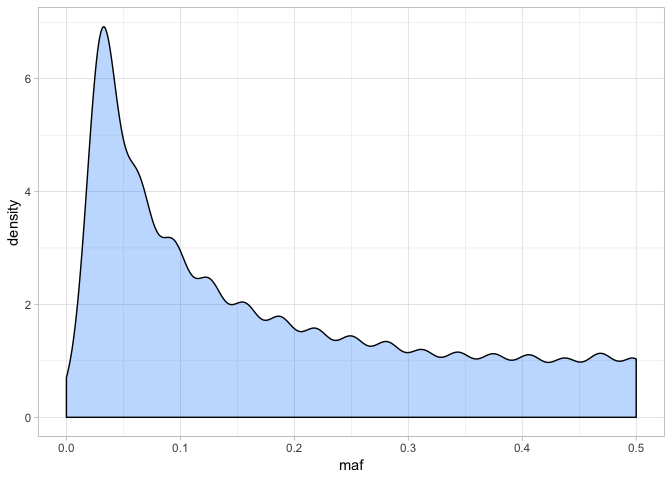
The distribution might look a little odd - this is partly because of the low number of individuals we have in the dataset (16), meaning there are only certain frequencies possible. Nonetheless, it is clear that a large number of variants have low frequency alleles. We can also look at the distribution in more detail:
summary(var_freq$maf)
##    Min. 1st Qu.  Median    Mean 3rd Qu.    Max.
##  0.0000  0.0625  0.1250  0.1788  0.2812  0.5000
The upper bound of the distribution is 0.5, which makes sense because if MAF was more than this, it wouldn’t be the MAF! How do we interpret MAF? It is an important measure because low MAF alleles may only occur in one or two individuals. It is possible that some of these low frequency alleles are in fact unreliable base calls - i.e. a source of error.
With 16 individuals, there are 28 alleles for a given site. Therefore MAF = 0.04 is equivalent to a variant occurring as one allele in a single individual (i.e. 28 * 0.04 = 1.12). Alternatively, an MAF of 0.1 would mean that any allele would need to occur at least twice (i.e. 28 * 0.1 = 2.8).
Setting MAF cutoffs is actually not that easy or straightforward. Hard MAF filtering (i.e. setting a high threshold) can severely bias estimation of the site frequency spectrum and cause problems with demographic analyses. Similarly, an excesss of low frequency, ‘singleton’ SNPs (i.e. only occurring in one individual) can mean you keep many uniformative loci in your dataset that make it hard to model things like population structure.
Usually then, it is best practice to produce one dataset with a good MAF threshold and keep another without any MAF filtering at all. For now however, we will set our MAF to 0.1
Individual based statistics
As well as a our per variant statistics we generated earlier, we also calculated some individual metrics too. WE can look at the distribution of these to get an idea whether some of our individuals have not sequenced or mapped as well as others. This is good practice to do with a new dataset. A lot of these statistics can be compared to other measures generated from the data (i.e. principal components as a measure of population structure) to see if they drive any apparent patterns in the data.
Mean depth per individual
First we will look at the distribution of mean depth among individuals. We read the data in with read_delim:
ind_depth <- read_delim("./cichlid_subset.idepth", delim = "\t",
                        col_names = c("ind", "nsites", "depth"), skip = 1)
Then we plot the distribution as a histogram using ggplot and geom_hist.
a <- ggplot(ind_depth, aes(depth)) + geom_histogram(fill = "dodgerblue1", colour = "black", alpha = 0.3)
a + theme_light()
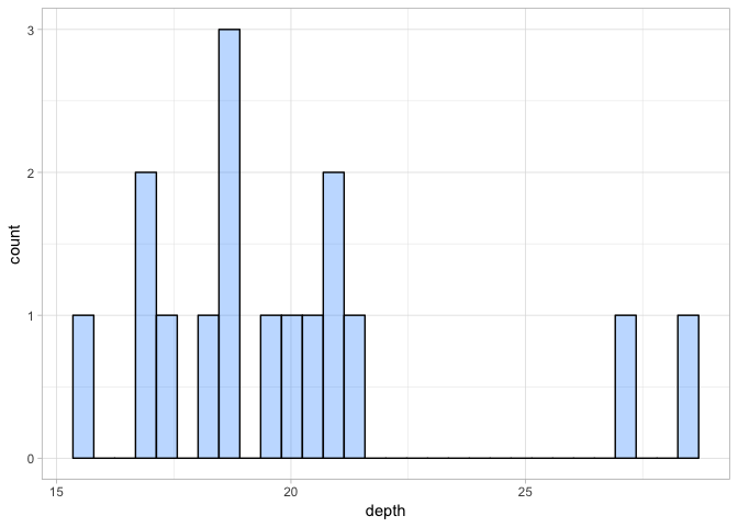
Because we are only plotting data for 16 individuals, the plot looks a little disjointed. While there is some evidence that some individuals were sequenced to a higher depth than others, there are no extreme outliers. So this doesn’t suggest any issue with individual sequencing depth.
Proportion of missing data per individual
Next we will look at the proportion of missing data per individual. We read in the data below:
ind_miss  <- read_delim("./cichlid_subset.imiss", delim = "\t",
                        col_names = c("ind", "ndata", "nfiltered", "nmiss", "fmiss"), skip = 1)
This is very similar to the missing data per site. Here we will focus on the fmiss column - i.e. the proportion of missing data.
a <- ggplot(ind_miss, aes(fmiss)) + geom_histogram(fill = "dodgerblue1", colour = "black", alpha = 0.3)
a + theme_light()
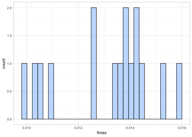
Again this shows us, the proportion of missing data per individual is very small indeed. It ranges from 0.01-0.16, so we can safely say our individuals sequenced well.
Heterozygosity and inbreeding coefficient per individual
ind_het <- read_delim("./cichlid_subset.het", delim = "\t",
           col_names = c("ind","ho", "he", "nsites", "f"), skip = 1)
a <- ggplot(ind_het, aes(f)) + geom_histogram(fill = "dodgerblue1", colour = "black", alpha = 0.3)
a + theme_light()
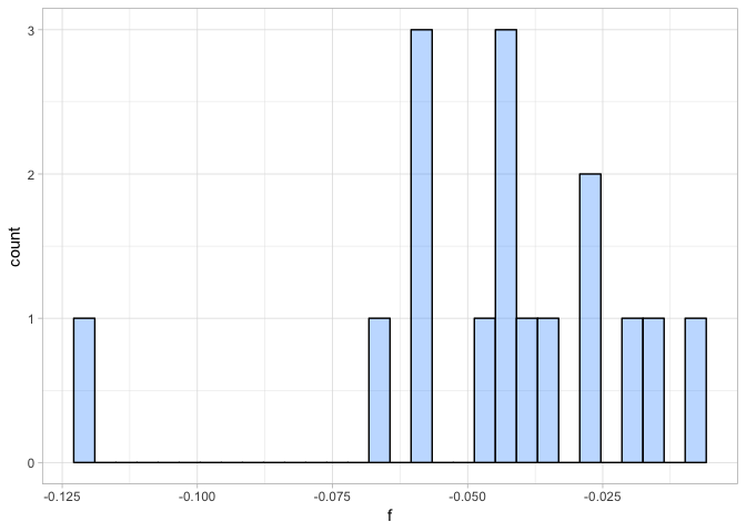
All individuals have a slightly negative inbreeding coefficient suggesting that we observed a bit less heterozygote genotypes in these individuals than we would expect under Hardy-Weinberg equilibrium. However, here we combined samples from four species and thus violate the assumption of Hardy-Weinberg equilibrium. We would expect slightly negative inbreeding coefficients due to the Wahlund-effect. Given that all individuals seem to show similar inbreeding coefficients, we are happy to keep all of them. None of them shows high levels of allelic dropout (strongly negative F) or DNA contamination (highly positive F).
Applying filters to the VCF
Now we have an idea of how to set out thresholds, we will do just that. First of all, we will set some simple variables in order to make our filtering command more straightforward.
VCF_IN=~/vcf/cichlid_full.vcf.gz
VCF_OUT=~/vcf/cichlid_full_filtered.vcf.gz
Then next we will set our chosen filters like so:
# set filters
MAF=0.1
MISS=0.9
QUAL=30
MIN_DEPTH=10
MAX_DEPTH=50
Finally we run the following vcftools command on the data to produce a filtered vcf. We will investigate the options as the filtering is running.
# move to the vcf directory
cd vcf
# perform the filtering with vcftools
vcftools --gzvcf $VCF_IN \
--remove-indels --maf $MAF --max-missing $MISS --minQ $QUAL \
--min-meanDP $MIN_DEPTH --max-meanDP $MAX_DEPTH \
--minDP $MIN_DEPTH --maxDP $MAX_DEPTH --recode --stdout | gzip -c > \
$VCF_OUT
What have we done here?
--gvcf- input path – denotes a gzipped vcf file--remove-indels- remove all indels (SNPs only)--maf- set minor allele frequency - 0.1 here--max-missing- set minimum non-missing data. A little counterintuitive - 0 is totally missing, 1 is none missing. Here 0.9 means we will tolerate 10% missing data.--minQ- this is just the minimum quality score required for a site to pass our filtering threshold. Here we set it to 30.--min-meanDP- the minimum mean depth for a site.--max-meanDP- the maximum mean depth for a site.--minDP- the minimum depth allowed for a genotype - any individual failing this threshold is marked as having a missing genotype.--maxDP- the maximum depth allowed for a genotype - any individual failing this threshold is marked as having a missing genotype.--recode- recode the output - necessary to output a vcf--stdout- pipe the vcf out to the stdout (easier for file handling)
Now, how many variants remain? There are two ways to examine this - look at the vcftools log or the same way we tried before.
cat out.log
bcftools view -H cichlid_full_filtered.vcf.gz | wc -l
You can see we have substantially filtered our dataset!