Demographic modeling with fastsimcoal2
fastsimcoal2 is an extremely flexible demographic modelling software developed by the group of Laurent Excoffier at University of Bern. It uses the site frequency spectrum (SFS) to fit model parameters to the observed data by performing coalescent simulations. You can find the manual and more information here and look at the lecture slides.
Preparing the input files
To run fastsimcoal2 we need three input files which are all named in a consistent way. They are all just plain text files.
- observed SFS -
${PREFIX}_jointDAFpop1_0.obs - template file defining the demographic model -
${PREFIX}.tpl - estimation file defining the parameters -
${PREFIX}.est
Note, you can find examples here.
Observed SFS
The observed SFS can be a derived SFS (i.e. also known as DAF or an unfolded SFS) if the ancestral state is unknown or a minor allele frequency SFS (i.e. MAF or folded SFS) otherwise. fastsimcoal2 will identify the kind of SFS by its name suffix and the command flag -m or -d. For a single population, it expects the name ${PREFIX}_DAFpop0.obs or ${PREFIX}_MAFpop0.obs.
For two populations, the file names should end with jointDAFpop1_0.obs or jointMAFpop1_0.obs. If more than two observed populations are used, pairwise MAFs or DAFs can be provided following the naming scheme above or a multidimensional SFS can be used ending with _DSFS.obs or _MSFS.obs and specifying the -multiSFS flag when running the program. See the fastsimcoal2 manual for further details. The .obs file can be generated with Arlequin, angsd, easySFS (as in this tutorial) or several other tools.
Template file
The template file describes the demographic model and the parameters of interest. Values that should be estimated (i.e. model parameters such as migration rate, splitting time etc) are given as different keywords. It is best practise to use capital letters for parameters names and it is important to avoid any names that are part of another parameter name or a function (e.g. log, min, FREQ).
As fastsimcoal2 is a coalescent simulator, all models need to be specified backwards in time. This means that the most recent event is specified first. The template file is best produced by modifying an example tpl file in a text editor.
In this tutorial, we will first write a model of two species that diverged in the face of gene flow and then evolved complete reproductive isolation. Unfortunately, we do not have a good estimate for the mutation rate, but we have an estimate for the (maximum possible) splitting time. Here we will set the split between the populations to 6000 generations.
Question for discussion: Why do we need to fix a parameter (e.g. splitting time) if we do not have a reliable mutation rate estimate?
Estimation file
All keywords introduced in the template file need to be defined in the estimation file. For each keyword, the parameter distribution (uniform or log-uniform) and search range (min and max) are given on a single line. Each parameter can be an integer or a float, as specified by a first indicator variable.
Lastly, complex parameters can be used to compute parameter values with simple operations such as computing the ratio between two simple parameters or specifying a parameter as the minimum of two parameters. In addition, for each simple or complex parameter, one needs to specify if the parameter value should be written into an output file or not.
As with the template file, the estimation file is best produced by modifying an example est file in a text editor.
Running fastsimcoal2
Once we have all input files ready, it is time to run fastsimcoal. In addition to the input files, we need to specify how many simulations and iterations fastsimcoal should perform, when to stop and how many threads (i.e. CPUs) can be used in parallel.
Let’s run fastsimcoal with our model of two populations. First we make a fastsimcoal directory and in that one a directory for our model of early_geneflow:
PREFIX="early_geneflow"
mkdir fastsimcoal
cd fastsimcoal
mkdir early_geneflow
cd early_geneflow
cp /home/data/fastsimcoal2/early_geneflow/* ./
fastsimcoal2 -t ${PREFIX}.tpl -e ${PREFIX}.est -m -0 -C 10 -n 10000 -L 40 -s 0 -M
This command runs fastsimcoal using a MAF (-m) while ignoring monomorphic sites (-0) and SFS entries with less than 10 SNPs (-C). This means that entries with less than 10 SNPs are pooled together. This option is useful when there are many entries in the observed SFS with few SNPs and with a limited number of SNPS to avoid overfitting.
fastsimcoal will also perform (-n) 10,000 coalescent simulations to approximate the expected SFS in each cycle and will run (-L) 40 optimization (ECM) cycles to estimate the parameters. The number of ECM cycles should be at least 20, better between 50 and 100. The number of coalescent simulations should ideally be something between 200,000 and 1,000,000 but to make it faster, we are now only running 10,000 simulations. We also specify (-M) that we want to perform parameter estimation. With -s 0, we can tell fastsimcoal to output SNPs.
Once fastsimcoal is finished, we can have a look at the output files.
It produced a folder called ${PREFIX} which contains a number of new files. The most relevant files are the following:
${PREFIX}.bestlhoods:file with the Maximum likelihood estimates for each parameter specified “output” in theestfile and the model likelihoods.${PREFIX}._jointMAFpop1_0.txt: file with the expected SFS obtained with the parameters that maximized the likelihood during optimization. This is needed to visually check the fit of the expected SFS to the observed SFS. This file has the same suffix as the observed SFS provided.${PREFIX}.simparam: file with an example of the settings to run the simulations. This is useful to check when you have errors. Many times errors in specification of models can be detected in this file.${PREFIX}_maxL.par: Model specification file with the best parameter estimates. It is basically the tpl file with the keywords replaced by estimated values. This file is useful if you want to simulate data under the best model using Arlequin.
Note, the bestlhoods file contains two different likelihoods: MaxObsLhood: is the maximum possible value for the likelihood if there was a perfect fit of the expected to the observed SFS, i.e. if the expected SFS was the relative observed SFS.
MaxEstLhood: is the maximum likelihood estimated according to the model parameters. It is obtained by using the observed SFS as the expected SFS when computing the likelihood, i.e., returning the value of the likelihood if there was a perfect fit between the expected and observed SFS.
The better the fit, the smaller the difference between MaxObsLhood and MaxEstLhood.
Finding the best parameter estimates
fastsimcoal2 should not just be run once because it might not find the global optimum of the best combination of parameter estimates right away. It is better to run it 100 times or more. Of these runs, select the one with the highest likelihood which is the run with the best fitting parameter estimates for this model.
Due to time constraints, we will only run this model 5 times. Note, I added the flag -q for “quiet” which reduces the amount of information fsc writes to stdout.
 for i in {1..5}
 do
   mkdir run$i
   cp ${PREFIX}.tpl ${PREFIX}.est ${PREFIX}_jointMAFpop1_0.obs run$i"/"
   cd run$i
   fastsimcoal2 -t ${PREFIX}.tpl -e ${PREFIX}.est -m -0 -C 10 -n 10000 -L 40 -s0 -M -q
   cd ..
 done
To find the best run, i.e. the run with the highest likelihood, or better the smallest difference between the maximum possible likelihood (MaxObsLhood) and the obtained likelihood (MaxEstLhood), we can check the .bestlhoods files.
cat run{1..5}/${PREFIX}/${PREFIX}.bestlhoods | grep -v MaxObsLhood | awk '{print NR,$8}' | sort -k 2
Note that NR in awk prints out the line number which here corresponds to the run number. $8 is the MaxEstLhood column and thus the likelihood we want to compare across different runs.
Joana wrote a script for you that automatically extracts the files of the best run and copies them into a new folder which it calls bestrun. Just run it in the directory where all the folders run are located:
fsc-selectbestrun.sh
Now modify the $PREFIX.tpl and $PREFIX.est files to specify different models and also rename the SFS to ${PREFIX}_jointDAFpop1_0.txt. Then run fastsimcoal2 for all models to see which one shows the best fit to the observed SFS.
Click here to see a possible solution.
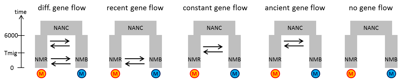
Early Geneflow (this is the model expalined in the example, gene flow right after the split and then no gene flow anymore, e.g. speciation with gene flow and then no gene flow anymore as reproductive isolation becomes strong):
tpl
est
No geneflow:
tpl
est
Recent geneflow (no gene flow intially after the split but gene flow in recent times, e.g. secondary contact scenario)
tpl
est
Different gene flow matrices (higher or lower gene flow right after the split than recently, e.g. initially higher gene flow then lower gene flow as reproductive isolation accumulates):
tpl
est
Constant gene flow (same gene flow strengths since the split until now):
tpl
est
Model comparison with AIC
In order to find the best model, the likelihoods of the best run of each model should be compared. Comparing raw likelihoods is problematic, because a model with more parameters will always tend to result in a better fit to the data. Therefore, the Akaike information criterium or AIC is typically calculated to determine if the models differ in their likelihoods accounting for the number of parameters in each model. Also for this you can use a script that is mostly based on R code by Vitor Sousa.
cd bestrun/
calculateAIC.sh early_geneflow
This script generates a file ${PREFIX}.AIC which contains the delta likelihood and the AIC value for that run.
Visualize the model fit
To visualize the fit of the simulated SFS to the data, we can use an R script that David Marques wrote - SFStools.r - which you can download here.
To visualize the model with the best parameter estimates, we can use one of Joana Meier’s R scripts - plotModel.r. There are also other options here.
SFStools.r -t print2D -i early_geneflow
plotModel.r -p early_geneflow -l NyerMak,PundMak
Now, let’s download the pdfs these scripts generated.
scp -i c1.pem user1@<ip>:~/fastsimcoal/early_geneflow/bestrun/*pdf ./
Model comparison with Likelihood distributions
One drawback of the composite likelihoods in model tests based on AIC is that it can overestimate the support for the most likely model if the SNPs are not independent (here they are not LD-pruned). Another way to infer if the models are really different and do not just differ because of stochasticity in the likelihood approximation, is to get likelihood distributions for each model. This is done by running each model with the best parameter values multple times (ideally about 100 times). The likelihoods will differ because fastsimcoal does not compute the likelihood but rather approximates it with simulations. If the ranges of likelihoods of two models overlap, it means that they do not differ significantly, i.e. provide an equally good fit to the observed data.
Let’s recompute the likelihood for the best run for the early_geneflow model.
PREFIX="early_geneflow"
cd ~/fastsimcoal/$PREFIX/bestrun

# create temporary obs file with name _maxL_MSFS.obs
cp ${PREFIX}_jointMAFpop1_0.obs ${PREFIX}_maxL_jointMAFpop1_0.obs

# Run fastsimcoal 20 times (in reality better 100 times) to get the likelihood of the observed SFS under the best parameter values with 1 mio simulated SFS.
for i in {1..20}
do
 fastsimcoal2 -i ${PREFIX}_maxL.par -n1000000 -m -q -0
 # Fastsimcoal will generate a new folder called ${model}_maxL and write files in there

 # collect the lhood values (Note that >> appends to the file, whereas > would overwrite it)
 sed -n '2,3p' ${PREFIX}_maxL/${PREFIX}_maxL.lhoods  >> ${PREFIX}.lhoods

 # delete the folder with results
 rm -r ${PREFIX}_maxL/
done
We would now repeat this for different models: ongoing gene flow, a model without gene flow, a model of secondary contact (recent gene flow) and a model with different amounts of gene flow in the past and in recent times.
Due to time constraints, we will give you the results of these models. They are in the same format as the folder we generated for the model with early gene flow. Load them into your modeling folder. Note, the -r flag stands for “recursive” and allows to also copy directories and their contents.
cp -r /home/data/fastsimcoal2/extramodels/* ~/fastsimcoal/
Now, let’s download the likelihoods and plot them:
scp -i c.pem user@<ip>:~/fastsimcoal/lhoods/* ./
On the local computer, we can plot the likelihoods as boxplots.
setwd()

# Read in the likelihoods
early_geneflow<-scan("early_geneflow.lhoods")
ongoing_geneflow<-scan("ongoing_geneflow.lhoods")
diff_geneflow<-scan("diff_geneflow.lhoods")
recent_geneflow<-scan("recent_geneflow.lhoods")
no_geneflow<-scan("no_geneflow.lhoods")

# Plot the likelihoods

par(mfrow=c(1,1))
boxplot(range = 0,diff_geneflow,recent_geneflow,early_geneflow,ongoing_geneflow,
        no_geneflow, ylab="Likelihood",xaxt="n")
axis(side=1,at=1:5, labels=c("early+recent","recent","early","constant","no"))
Similarly, we should compare the AIC values and see if AIC suggests that the second-best model is significantly less good than the best model. Given that we already used the calculateAIC.r script to compute AIC values, this can easily be done.
for i in */bestrun/*AIC
do
echo -e `basename $i`"\t"`tail -n $i` >> allmodels.AIC
done
Now that we know which of the models is the best one, we can do some bootstrapping to figure out how certain we are in our parameter estimates. We will use block-bootstrapping to account for linkage between SNPs:
# Get all lines with genomic data
zgrep -v "^#" $PREFIX.vcf > $PREFIX.allSites

# Get the header
zgrep "^#" $PREFIX.vcf > header

# get 100 files with 4338 sites each (number 101 removed due to only 90 sites)
split -l 4338 $PREFIX.allSites $PREFIX.sites.

# Generate 50 files each with randomly concatenated blocks and compute the SFS for each:
for i in {1..50}
do
  # Make a new folder for each bootstrapping iteration:
  mkdir bs$i
  cd bs$i

  # Add the header to our new bootstrapped vcf file
  cat ../header > $PREFIX.bs.$i.vcf
  # Randomly add 100 blocks
  for r in {1..100}
  do
    cat `shuf -n1 -e ../$PREFIX.sites.*` >> ${PREFIX}.bs.$i.vcf
  done
  # Compress the vcf file again
  gzip ${PREFIX}.bs.$i.vcf

  # Make an SFS from the new bootstrapped file
  easySFS.py -i ${PREFIX}.bs.$i.vcf.gz -p pop_file -a -f --proj 8,8

  # Copy the observed SFS file into this folder renaming it to match the .tpl prefix
  cp ../${PREFIX}_jointDAFpop1_0.obs  ${PREFIX}.bs.${i}_jointDAFpop1_0.obs

  # Say that it is finished with iteration $i
  echo bs$i" ready"

  cd ..
done
Now we would run the parameter estimation under the best model 100 times with each of these boostrapped SFS. This would take very long.
for bs in {1..50}
do
  cd bs$bs
  # Run fastsimcoal 100 times:
  for i in {1..100}
  do
    mkdir run$i
    cd run$i
    cp ${PREFIX}.bs.$bs.* ./
    fastsimcoal2 -t ${PREFIX}.bs.$bs.tpl -e ${PREFIX}.bs.$bs.est -m -0 -C 10 -n 10000 -L 40 -s0 -M -q
    cd ..
  done
  # Find the best run:
  fsc-selectbestrun.sh

  cd ..
done
Now we can compute the confidence interval using the parameter estimates of the bestrun files of all bootstrapping replicates, e.g. with the R package boot.